Anscombe’s Quartet

Anscombe’s Quartet, known as the “Anscombe’s Test,” consists of four datasets with very similar descriptive statistics but visually distinct characteristics. These quartets serve as an enlightening example of the importance of visualizing data before drawing conclusions.

In this post, we will delve into how to calculate and visualize Anscombe’s Quartet using R and the powerful ggplot2 library. We’ll also use custom functions to generate these quartets and analyze them.

Anscombe’s Quartet was created by the statistician Francis Anscombe in 1973 to underscore the importance of data visualization before analysis. Despite having similar statistics, these datasets exhibit significantly different visual behaviors. Let’s see how R and ggplot2 help us explore them.

To get started, we need to load some libraries:

library(data.table)
library(ggplot2)
library(patchwork)

Anscombe’s Quartet comprises four datasets, each with 11 data points. Here’s a brief overview of the quartet:

• Dataset 1: A straightforward linear relationship between X and Y.

• Dataset 2: A linear relationship with an outlier.

• Dataset 3: A linear relationship with one point substantially different from the others.

• Dataset 4: A non-linear relationship.

(see Rpubs page)

library(datasets)
library(ggplot2)
library(dplyr)

Attaching package: 'dplyr'

The following objects are masked from 'package:data.table':

    between, first, last

The following objects are masked from 'package:stats':

    filter, lag

The following objects are masked from 'package:base':

    intersect, setdiff, setequal, union

library(tidyr)
datasets::anscombe

   x1 x2 x3 x4    y1   y2    y3    y4
1  10 10 10  8  8.04 9.14  7.46  6.58
2   8  8  8  8  6.95 8.14  6.77  5.76
3  13 13 13  8  7.58 8.74 12.74  7.71
4   9  9  9  8  8.81 8.77  7.11  8.84
5  11 11 11  8  8.33 9.26  7.81  8.47
6  14 14 14  8  9.96 8.10  8.84  7.04
7   6  6  6  8  7.24 6.13  6.08  5.25
8   4  4  4 19  4.26 3.10  5.39 12.50
9  12 12 12  8 10.84 9.13  8.15  5.56
10  7  7  7  8  4.82 7.26  6.42  7.91
11  5  5  5  8  5.68 4.74  5.73  6.89

summary(anscombe)

       x1             x2             x3             x4           y1        
 Min.   : 4.0   Min.   : 4.0   Min.   : 4.0   Min.   : 8   Min.   : 4.260  
 1st Qu.: 6.5   1st Qu.: 6.5   1st Qu.: 6.5   1st Qu.: 8   1st Qu.: 6.315  
 Median : 9.0   Median : 9.0   Median : 9.0   Median : 8   Median : 7.580  
 Mean   : 9.0   Mean   : 9.0   Mean   : 9.0   Mean   : 9   Mean   : 7.501  
 3rd Qu.:11.5   3rd Qu.:11.5   3rd Qu.:11.5   3rd Qu.: 8   3rd Qu.: 8.570  
 Max.   :14.0   Max.   :14.0   Max.   :14.0   Max.   :19   Max.   :10.840  
       y2              y3              y4        
 Min.   :3.100   Min.   : 5.39   Min.   : 5.250  
 1st Qu.:6.695   1st Qu.: 6.25   1st Qu.: 6.170  
 Median :8.140   Median : 7.11   Median : 7.040  
 Mean   :7.501   Mean   : 7.50   Mean   : 7.501  
 3rd Qu.:8.950   3rd Qu.: 7.98   3rd Qu.: 8.190  
 Max.   :9.260   Max.   :12.74   Max.   :12.500  

anscombe_tidy <- anscombe %>%
    mutate(observation = seq_len(n())) %>%
    gather(key, value, -observation) %>%
    separate(key, c("variable", "set"), 1, convert = TRUE) %>%
    mutate(set = c("I", "II", "III", "IV")[set]) %>%
    spread(variable, value)

head(anscombe_tidy)

  observation set  x    y
1           1   I 10 8.04
2           1  II 10 9.14
3           1 III 10 7.46
4           1  IV  8 6.58
5           2   I  8 6.95
6           2  II  8 8.14

ggplot(anscombe_tidy, aes(x, y)) +
    geom_point() +
    facet_wrap(~ set) +
    geom_smooth(method = "lm", se = FALSE)

`geom_smooth()` using formula = 'y ~ x'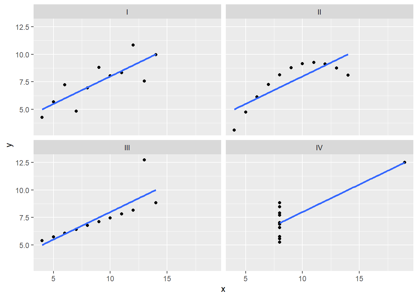

Now, let’s integrate your custom R code and examples to generate and visualize Anscombe’s Quartet:

library(vtable)

Loading required package: kableExtra

Attaching package: 'kableExtra'

The following object is masked from 'package:dplyr':

    group_rows

library(kableExtra)
library(patchwork)


# Note: Function to generate Anscombe's Quartet datasets for x2 we need a trick that can be also improved but for now as a brutal approx works


plotreg <- function(df) {
  formula <- y ~ x
  
  ggplot(df, aes(x = x, y = y)) +
    geom_point(aes(size = 1), alpha = 0.3) +
    geom_smooth(method = "lm", formula = formula, se = TRUE) +
    coord_cartesian(xlim = c(4, 19), ylim = c(4, 14)) +  # Imposta i limiti di x e y
    theme_light(base_size = 10) +
    theme(legend.position = "none")
}

generate_noisy_points <- function(x, y, noise_level = 0.1) {
  n <- length(x)
  
  # Generate random noise for x and y separately
  noise_x <- rnorm(n, mean = 0, sd = noise_level)
  noise_y <- rnorm(n, mean = 0, sd = noise_level)
  
  # Ensure that the sum of noise on x and y is approximately zero
  noise_x <- noise_x - mean(noise_x)
  noise_y <- noise_y - mean(noise_y)
  
  # Add noise to the original data
  x_noisy <- x + noise_x
  y_noisy <- y + noise_y
  
  return(data.frame(x = x_noisy, y = y_noisy))
}

# Function to generate approximated points with an option to add noise
generate_approximated_points <- function(n, x, y, noise_level = 0) {
  # Create a new interpolation based on the original data
  interpolated_values <- approx(x, y, xout = seq(min(x), max(x), length.out = n))
  
  # Extract the interpolated points
  x_interp <- interpolated_values$x
  y_interp <- interpolated_values$y
  
  # Add noise if needed
  if (noise_level > 0) {
    noise <- rnorm(n, mean = 0, sd = noise_level)
    x_interp <- x_interp + noise
    y_interp <- y_interp + noise
  }
  
  # Return the approximated points
  return(data.frame(x = x_interp, y = y_interp))
}


multians <- function(npoints = 11, anscombe) {
  x1 <- anscombe$x1
  x2 <- anscombe$x2
  x3 <- anscombe$x3
  x4 <- anscombe$x4
  y1 <- anscombe$y1
  y2 <- anscombe$y2
  y3 <- anscombe$y3
  y4 <- anscombe$y4

  ## Generate Quartet 1 ##
  x_selected <- c(x1[2], x1[4], x1[11])
  y_selected <- c(y1[2], y1[4], y1[11])

  # Calculate the linear regression
  linear_model <- lm(y_selected ~ x_selected)

  # Extract coefficients of the line
  intercept <- coef(linear_model)[1]
  slope <- coef(linear_model)[2]

  # Create a sinusoidal curve above or below the line
  x_sin <- seq(min(x1), max(x1), length.out = npoints)  # x range for the sinusoid
  amplitude <- 1  # Amplitude of the sinusoid
  frequency <- 4  # Frequency of the sinusoid
  phase <- pi / 2  # Phase of the sinusoid (for rotation)
  sinusoid <- amplitude * sin(2 * pi * frequency * (x_sin - min(x1)) / (max(x1) - min(x1)) + phase)

  # Generate points above or below the line
  y_sin <- slope * x_sin + intercept + sinusoid
  df1 <- data.frame(x = x_sin, y = y_sin)

  ## Generate Quartet 2 ##
  n_points_approximated <- npoints
  noise_level <- 0.1

  # Generate approximated points
  approximated_points <- generate_approximated_points(n_points_approximated, x2, y2, noise_level = 0.1)

  # Add noise to the approximated points
  noisy_approximated_points <- generate_noisy_points(approximated_points$x, approximated_points$y, noise_level)

  # Now, you have noisy approximated points in df2
  df2 <- data.frame(x = noisy_approximated_points$x, y = noisy_approximated_points$y)

  ## Generate Quartet 3 ##
  lm_model <- lm(y3 ~ x3, subset = -c(3))
  x_generated <- seq(min(x3), max(x3), length.out = npoints)
  y_generated <- predict(lm_model, newdata = data.frame(x3 = x_generated))

  x_outlier <- 13
  y_outlier <- 12.74
  x_generated <- c(x_generated, x_outlier)
  y_generated <- c(y_generated, y_outlier)

  df3 <- data.frame(x = x_generated, y = y_generated)

  ## Generate Quartet 4 ##
  
  y4[9]
  x <- c(rep(min(x4),npoints))
  y <- c(seq(min(y4[-8]), max(y4[-8]), length.out = (npoints)))
  x_new = c(x,x4[8])
  y_new = c(y,y4[8])
  df4 <- data.frame(x = x_new, y = y_new)

  return(list(df1 = df1, df2 = df2, df3 = df3, df4 = df4))
}



# Generate and plot Quartet 1
t1 <- multians(33,anscombe)

p1 <- plotreg(t1$df1)
p3 <- plotreg(t1$df3)
p4 <- plotreg(t1$df4)
p2 <- plotreg(t1$df2)

(p1 | p2) / (p3 | p4)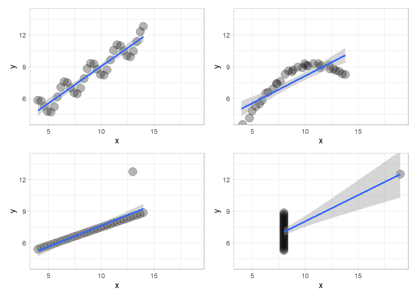

# Example of eight summaries (replace them with your own)
summary1 <- st(t1$df1)
summary5 <- st(data.frame(anscombe$x1,anscombe$y1))

summary2 <- st(t1$df2)
summary6 <- st(data.frame(anscombe$x2,anscombe$y2))

summary3 <- st(t1$df3)
summary7 <- st(data.frame(anscombe$x3,anscombe$y3))

summary4 <- st(t1$df4)
summary8 <- st(data.frame(anscombe$x4,anscombe$y4))


summary1 

Summary Statistics

Variable	N	Mean	Std. Dev.	Min	Pctl. 25	Pctl. 75	Max
x	33	9	3	4	6.5	12	14
y	33	8.3	2.2	4.7	6.5	10	13

summary5 

Summary Statistics

Variable	N	Mean	Std. Dev.	Min	Pctl. 25	Pctl. 75	Max
anscombe.x1	11	9	3.3	4	6.5	12	14
anscombe.y1	11	7.5	2	4.3	6.3	8.6	11

summary2 

Summary Statistics

Variable	N	Mean	Std. Dev.	Min	Pctl. 25	Pctl. 75	Max
x	33	9	3	4	6.5	11	14
y	33	7.6	1.8	3	6.6	8.9	9.3

summary6 

Summary Statistics

Variable	N	Mean	Std. Dev.	Min	Pctl. 25	Pctl. 75	Max
anscombe.x2	11	9	3.3	4	6.5	12	14
anscombe.y2	11	7.5	2	3.1	6.7	8.9	9.3

summary3

Summary Statistics

Variable	N	Mean	Std. Dev.	Min	Pctl. 25	Pctl. 75	Max
x	34	9.1	3.1	4	6.6	12	14
y	34	7.3	1.4	5.4	6.3	8.1	13

summary7 

Summary Statistics

Variable	N	Mean	Std. Dev.	Min	Pctl. 25	Pctl. 75	Max
anscombe.x3	11	9	3.3	4	6.5	12	14
anscombe.y3	11	7.5	2	5.4	6.2	8	13

summary4 

Summary Statistics

Variable	N	Mean	Std. Dev.	Min	Pctl. 25	Pctl. 75	Max
x	34	8.3	1.9	8	8	8	19
y	34	7.2	1.4	5.2	6.2	8	12

summary8

Summary Statistics

Variable	N	Mean	Std. Dev.	Min	Pctl. 25	Pctl. 75	Max
anscombe.x4	11	9	3.3	8	8	8	19
anscombe.y4	11	7.5	2	5.2	6.2	8.2	12

Anscombe’s Quartet is a powerful reminder that descriptive statistics alone may not reveal the complete story of your data. Visualization is a crucial tool in data analysis, helping you uncover patterns, outliers, and unexpected relationships that numbers alone might miss.

(Szafir 2018; Anscombe 1973)

References

Anscombe, F. J. 1973. “Graphs in Statistical Analysis.” The American Statistician 27 (1): 17–21. http://www.jstor.org/stable/2682899.

Szafir, Danielle Albers. 2018. “The Good, the Bad, and the Biased: Five Ways Visualizations Can Mislead (and How to Fix Them).” Interactions 25 (4): 26–33. https://doi.org/10.1145/3231772.