Exploring Card Shuffling: A Visual Journey

Today, we embark on a visual exploration of card shuffling, delving into a captivating technique known as the Faro shuffle. Unlike conventional shuffling, the Faro shuffle promises not just randomness but a mathematical symphony that unfolds card by card, a dance that echoes with the precision of numbers.

In the quest to unravel the intricacies of card shuffling, we turn to the Faro shuffle, a technique that mimics the graceful dance of cards. The accompanying R code brings this technique to life, allowing us to simulate the position of the ace of hearts after multiple Faro shuffles.

# Function to perform a faro shuffle on a deck of cards
faro <- function(deck, num_shuffles) {
  for (i in 1:num_shuffles) {
    half1 <- deck[1:(length(deck)/2)]
    half2 <- deck[(length(deck)/2 + 1):length(deck)]
    deck <- c()
    for (j in 1:length(half1)) {
      deck <- c(deck, half1[j], half2[j])
    }
  }
  return(deck)
}

Here, the faro function is defined to simulate the Faro shuffle. It takes a deck of cards (deck) and the number of shuffles to perform (num_shuffles). The function iterates through the halves of the deck, interleaving the cards to simulate the Faro shuffle. This process is repeated for the specified number of shuffles.

# Install the required packages if not already installed
if (!requireNamespace("ggplot2", quietly = TRUE)) {
  install.packages("ggplot2")
}

# Load the necessary packages
library(ggplot2)

# Function to simulate the position of the ace of hearts after shuffling
simulate_ace_of_hearts_position <- function(num_shuffles, num_simulations) {
  original_deck <- 1:52
  ace_position <- numeric(num_simulations)
  
  for (i in 1:num_simulations) {
    shuffled_deck <- faro(original_deck, num_shuffles)
    ace_position[i] <- which(shuffled_deck == 12)
  }
  
  return(ace_position)
}

# Simulation parameters
num_shuffles_list <- seq(1, 30, by = 1)
num_simulations <- 100

# Run the simulation
ace_positions <- lapply(num_shuffles_list, function(num_shuffles) {
  simulate_ace_of_hearts_position(num_shuffles, num_simulations)
})

# Prepare data for the plot
df <- data.frame(
  Num_Shuffles = rep(num_shuffles_list, each = num_simulations),
  Ace_Position = unlist(ace_positions)
)

# Create a line plot with a ribbon in ggplot2
ggplot(df, aes(x = Num_Shuffles, y = Ace_Position)) +
  geom_line() +
  geom_ribbon(aes(ymin = Ace_Position - 5, ymax = Ace_Position + 5), fill = "lightblue", alpha = 0.3) +
  geom_text(aes(label = Ace_Position), vjust = -0.5, hjust = 0.5, size = 3) +
  labs(title = "Ace of Hearts Position relative to Initial Position",
       x = "Number of Shuffles",
       y = "Ace of Hearts Position") +
  theme_minimal()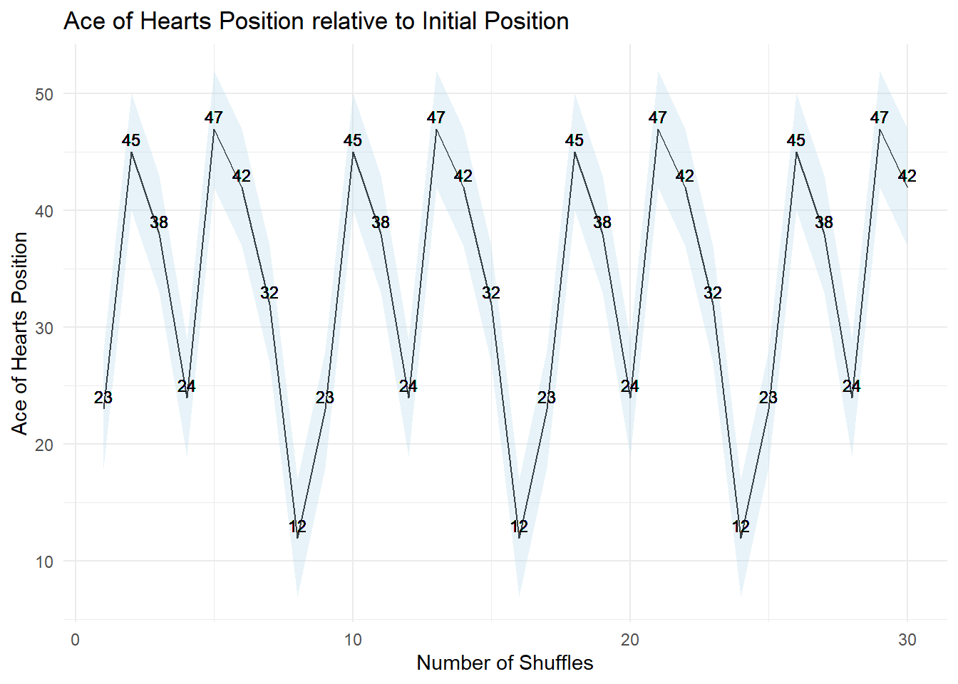

In the simulation parameters section, we define the number of Faro shuffles to explore (num_shuffles_list) and the number of simulations to run for each shuffle scenario (num_simulations). The resulting dataframe (’df’) contains the number of shuffles and the corresponding positions of the ace of hearts after simulation.Finallym the code utilizes ggplot2 to create a line plot with a ribbon that represents the range of possible ace of hearts positions after each Faro shuffle. The resulting visualization allows us to witness the mesmerizing journey of the ace of hearts through the rhytmic Faro shuffle.

Through this visual exploration, we gain insights into the inherent randomness of card shuffling. The fluctuating position of the ace of hearts highlights the complex interplay of probability and chance in card games.

Feel free to experiment with the provided R code, adjusting parameters and exploring different aspects of card shuffling. The visual representation serves as a captivating way to understand the nuances of this seemingly simple yet intriguing process.