Unraveling the DnD Dice Duel Riddle with Monte Carlo Simulation in R
R
Fun
Author
Giorgio Luciano and ChatGPT 3.5
Published
January 14, 2024
Embark on a journey into the realm of Dungeons & Dragons as we unravel a captivating fiddle riddle involving a dice duel. Using the power of the R programming language and the Monte Carlo simulation method, we’ll simulate the outcomes of duels between two players, each armed with a bag containing six distinct DnD dice. Prepare to explore the fascinating world of probability and randomness! See the riddle posted here by Fiddler on the Proof
At a table sit two individuals, each equipped with a bag housing six DnD dice: a d4, a d6, a d8, a d10, a d12, and a d20. The challenge is to randomly select one die from each bag and roll them simultaneously. For example, if a d4 and a d12 are chosen, both players roll their respective dice, hoping for fortuitous results. Monte Carlo Simulation in R:
To confront this enigma, we turn to the Monte Carlo method. The following R code snippet initiates a simulation of multiple dice duels, offering a glimpse into the complexities of DnD dice outcomes.
we can break down the analysis into different cases:
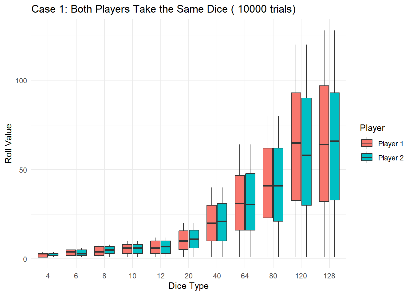
Case 1: Both players take the same type of dice.
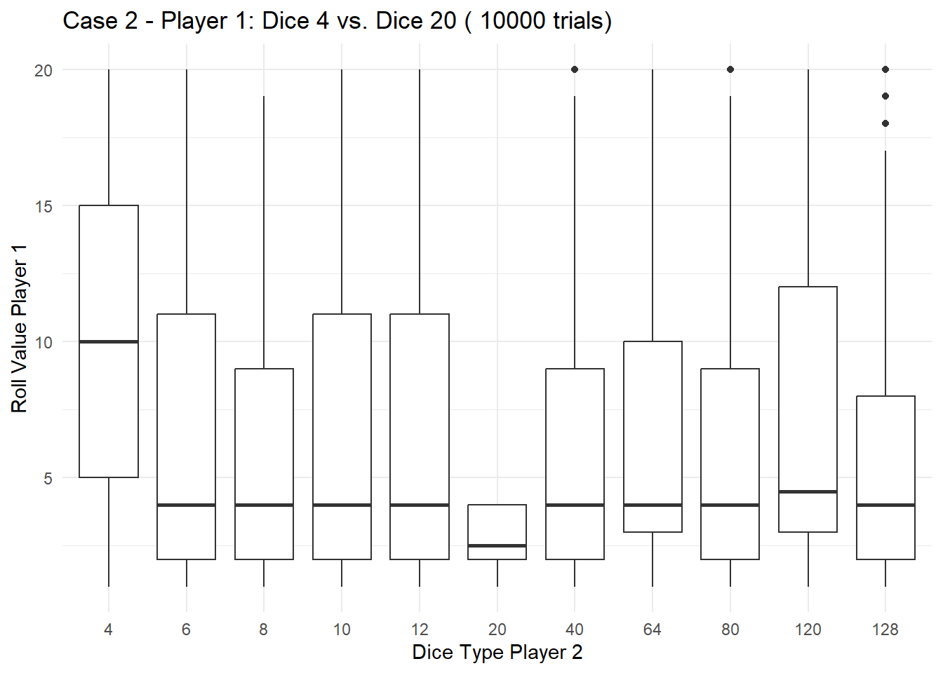
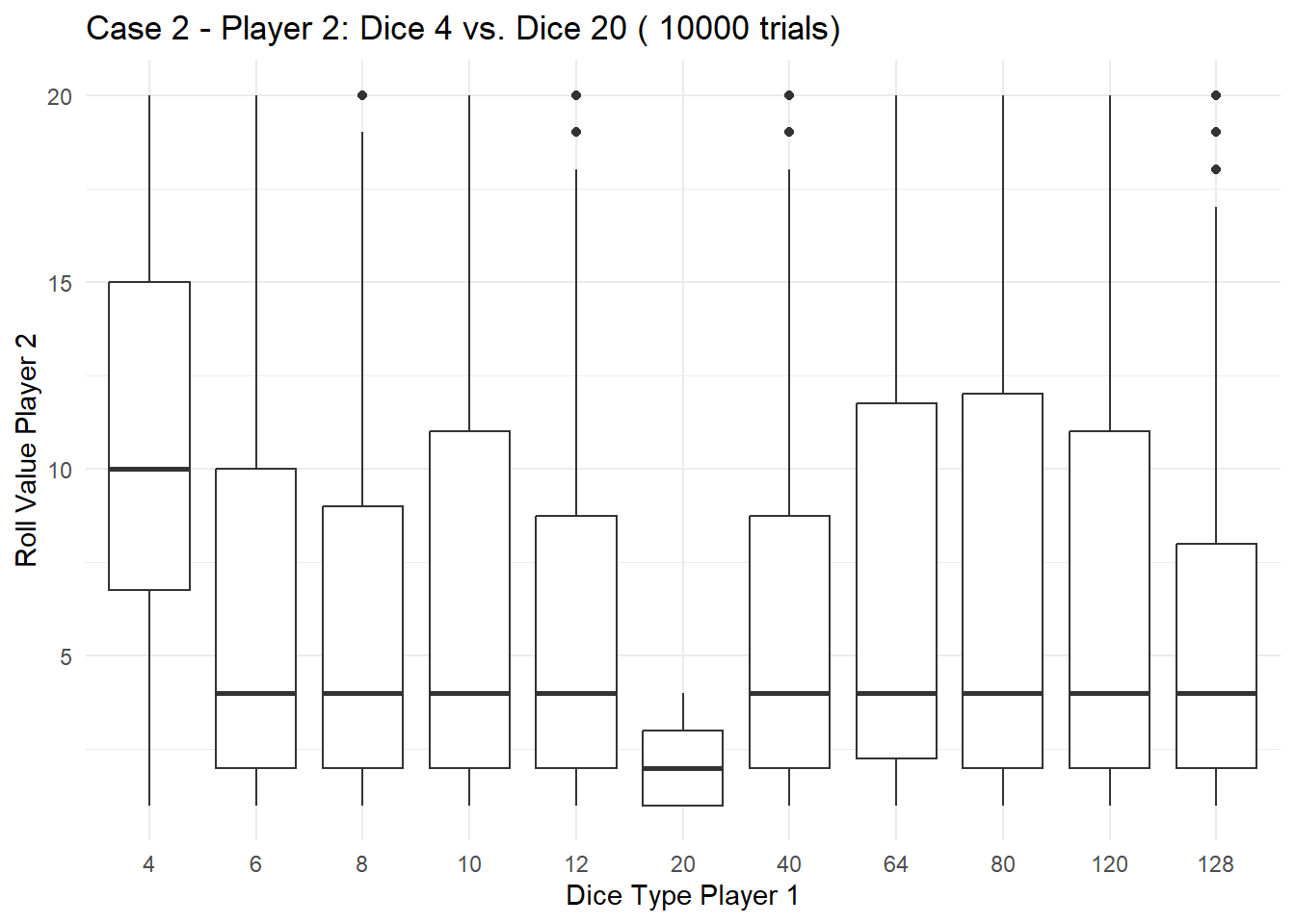
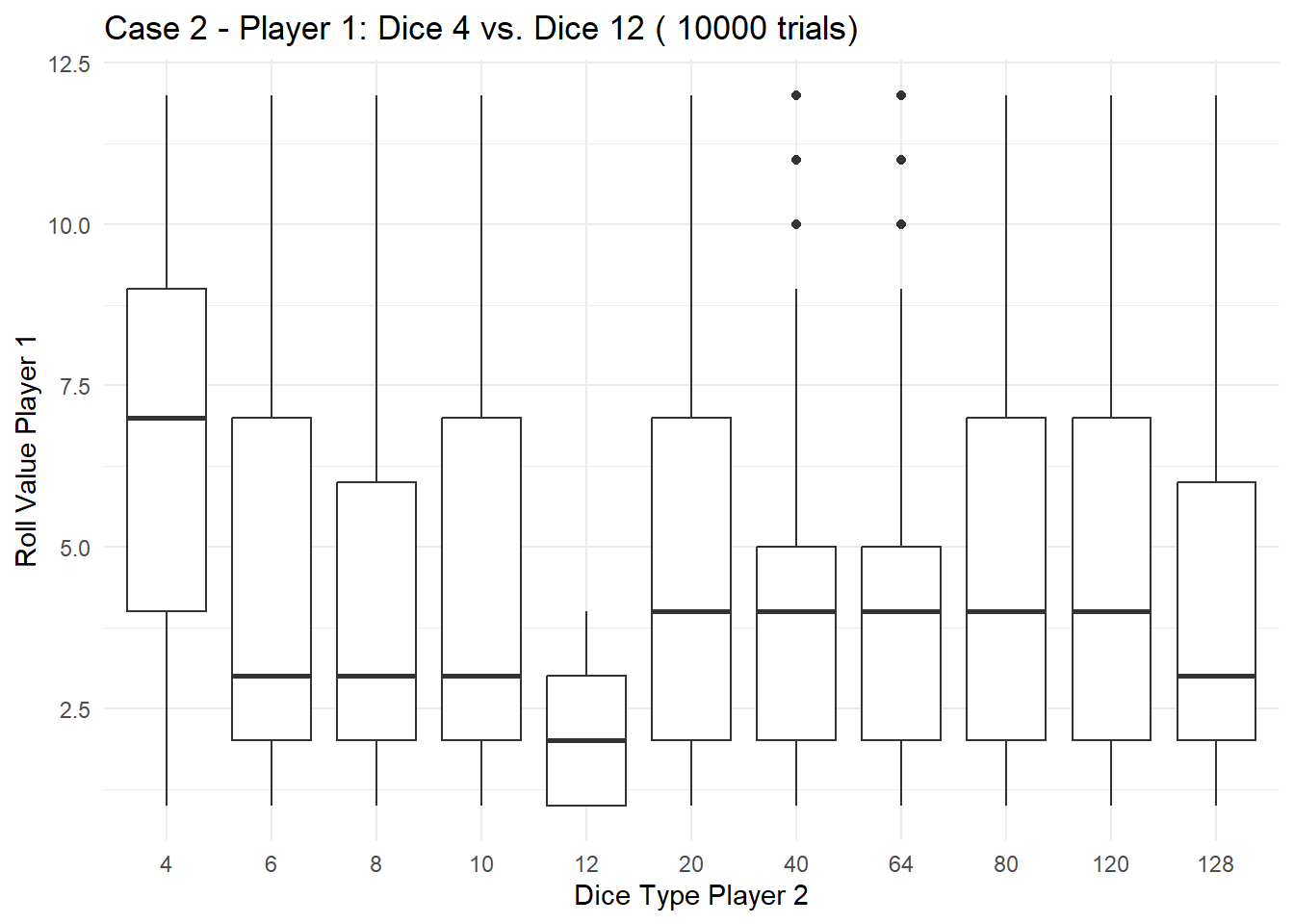
Case 2: Both players take different types of dice (without repetition of the same combination).
We’ll generate plots for each case and then provide a summary of the results. Here’s the code:
library(ggplot2)# Function to simulate a single dice duel with both players taking the same type of dicesimulate_same_dice_duel <-function() { dice_type <-sample(c(4, 6, 8, 10, 12,20,40,64,80,120,128), 1) roll_player1 <-sample(1:dice_type, 1) roll_player2 <-sample(1:dice_type, 1)return(c(dice_type, roll_player1, dice_type, roll_player2))}# Function to simulate a single dice duel with both players taking different types of dicesimulate_different_dice_duel <-function() { dice_types <-sample(c(4, 6, 8, 10, 12,20,40,64,80,120,128), 2, replace =FALSE) roll_player1 <-sample(1:dice_types[1], 1) roll_player2 <-sample(1:dice_types[2], 1)return(c(dice_types[1], roll_player1, dice_types[2], roll_player2))}# Monte Carlo simulation for both casesnum_trials <-10000# Case 1: Both players take the same type of dicesame_dice_simulation_results <-replicate(num_trials, simulate_same_dice_duel())same_dice_data <-data.frame(Player =rep(c("Player 1", "Player 2"), each =ncol(same_dice_simulation_results)),Dice_Type =rep(same_dice_simulation_results[1, ], 2),Roll_Value =as.integer(c(same_dice_simulation_results[2, ], same_dice_simulation_results[4, ])))# Visualize the results for Case 1 using ggplot2ggplot(same_dice_data, aes(x =factor(Dice_Type), y = Roll_Value, fill = Player)) +geom_boxplot() +labs(title =paste("Case 1: Both Players Take the Same Dice (", num_trials, "trials)"),x ="Dice Type",y ="Roll Value",fill ="Player") +theme_minimal()
# Case 2: Both players take different types of dicedifferent_dice_simulation_results <-replicate(num_trials, simulate_different_dice_duel())different_dice_data <-data.frame(Player =rep(c("Player 1", "Player 2"), each =ncol(different_dice_simulation_results)),Dice_Type_Player1 =rep(different_dice_simulation_results[1, ], 2),Roll_Value_Player1 =as.integer(c(different_dice_simulation_results[2, ])),Dice_Type_Player2 =rep(different_dice_simulation_results[3, ], 2),Roll_Value_Player2 =as.integer(c(different_dice_simulation_results[4, ])))# Visualize the results for Case 2 - Player 1 (Dice 4 vs. Dice 20)ggplot(subset(different_dice_data, Dice_Type_Player1 %in%c(4, 20)), aes(x =factor(Dice_Type_Player2), y = Roll_Value_Player1)) +geom_boxplot() +labs(title =paste("Case 2 - Player 1: Dice 4 vs. Dice 20 (", num_trials, "trials)"),x ="Dice Type Player 2",y ="Roll Value Player 1") +theme_minimal()
# Visualize the results for Case 2 - Player 2 (Dice 4 vs. Dice 20)ggplot(subset(different_dice_data, Dice_Type_Player2 %in%c(4, 20)), aes(x =factor(Dice_Type_Player1), y = Roll_Value_Player2)) +geom_boxplot() +labs(title =paste("Case 2 - Player 2: Dice 4 vs. Dice 20 (", num_trials, "trials)"),x ="Dice Type Player 1",y ="Roll Value Player 2") +theme_minimal()
# Visualize the results for Case 2 - Player 1 (Dice 4 vs. Dice 12)ggplot(subset(different_dice_data, Dice_Type_Player1 %in%c(4, 12)), aes(x =factor(Dice_Type_Player2), y = Roll_Value_Player1)) +geom_boxplot() +labs(title =paste("Case 2 - Player 1: Dice 4 vs. Dice 12 (", num_trials, "trials)"),x ="Dice Type Player 2",y ="Roll Value Player 1") +theme_minimal()
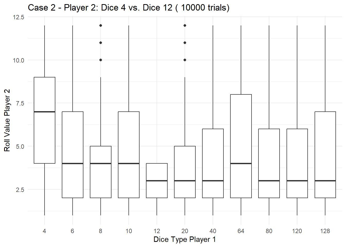
# Visualize the results for Case 2 - Player 2 (Dice 4 vs. Dice 12)ggplot(subset(different_dice_data, Dice_Type_Player2 %in%c(4, 12)), aes(x =factor(Dice_Type_Player1), y = Roll_Value_Player2)) +geom_boxplot() +labs(title =paste("Case 2 - Player 2: Dice 4 vs. Dice 12 (", num_trials, "trials)"),x ="Dice Type Player 1",y ="Roll Value Player 2") +theme_minimal()
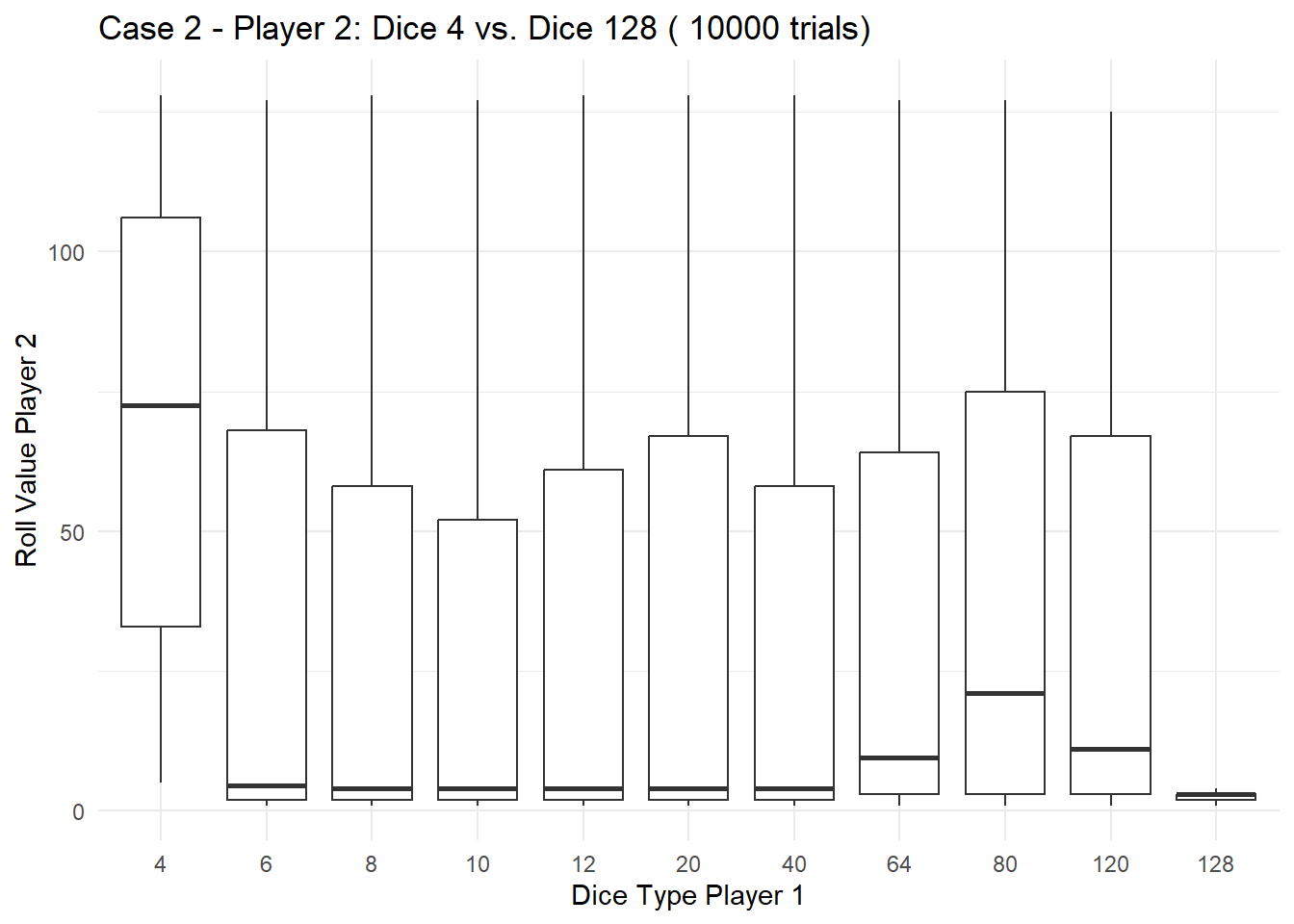
# Visualize the results for Case 2 - Player 2 (Dice 4 vs. Dice 128)ggplot(subset(different_dice_data, Dice_Type_Player2 %in%c(4, 128)), aes(x =factor(Dice_Type_Player1), y = Roll_Value_Player2)) +geom_boxplot() +labs(title =paste("Case 2 - Player 2: Dice 4 vs. Dice 128 (", num_trials, "trials)"),x ="Dice Type Player 1",y ="Roll Value Player 2") +theme_minimal()
# Summarize the results for Case 1 (Same Dice)summary_case1 <-table(same_dice_data$Roll_Value)# Summarize the results for Case 2 (Different Dice)summary_case2 <-table(different_dice_data$Roll_Value_Player1 == different_dice_data$Roll_Value_Player2)# Display summariescat("\nSummary of Case 1 - Same Dice:\n")
Through the marriage of R programming and Monte Carlo simulation, we’ve successfully deciphered the intricacies of the DnD dice duel riddle. Whether you’re a seasoned tabletop gamer or a data science enthusiast, this approach serves as a versatile tool for exploring and comprehending complex scenarios governed by chance. As you embark on your own coding adventures, may the rolls be ever in your favor! Happy coding!